Ever wondered why your paycheck seems to evaporate faster in certain zip codes across America? It’s not just your imagination playing tricks on you. The truth is, where you live can have a significant impact on your financial well-being, and that’s where the concept of High Cost of Living (HCOL) areas comes into play.
Let’s dive into the world of HCOL and explore how it affects our daily lives. HCOL refers to regions where the cost of basic necessities like housing, food, and transportation is substantially higher than the national average. Understanding these areas is crucial for anyone looking to make informed decisions about where to live, work, or invest.
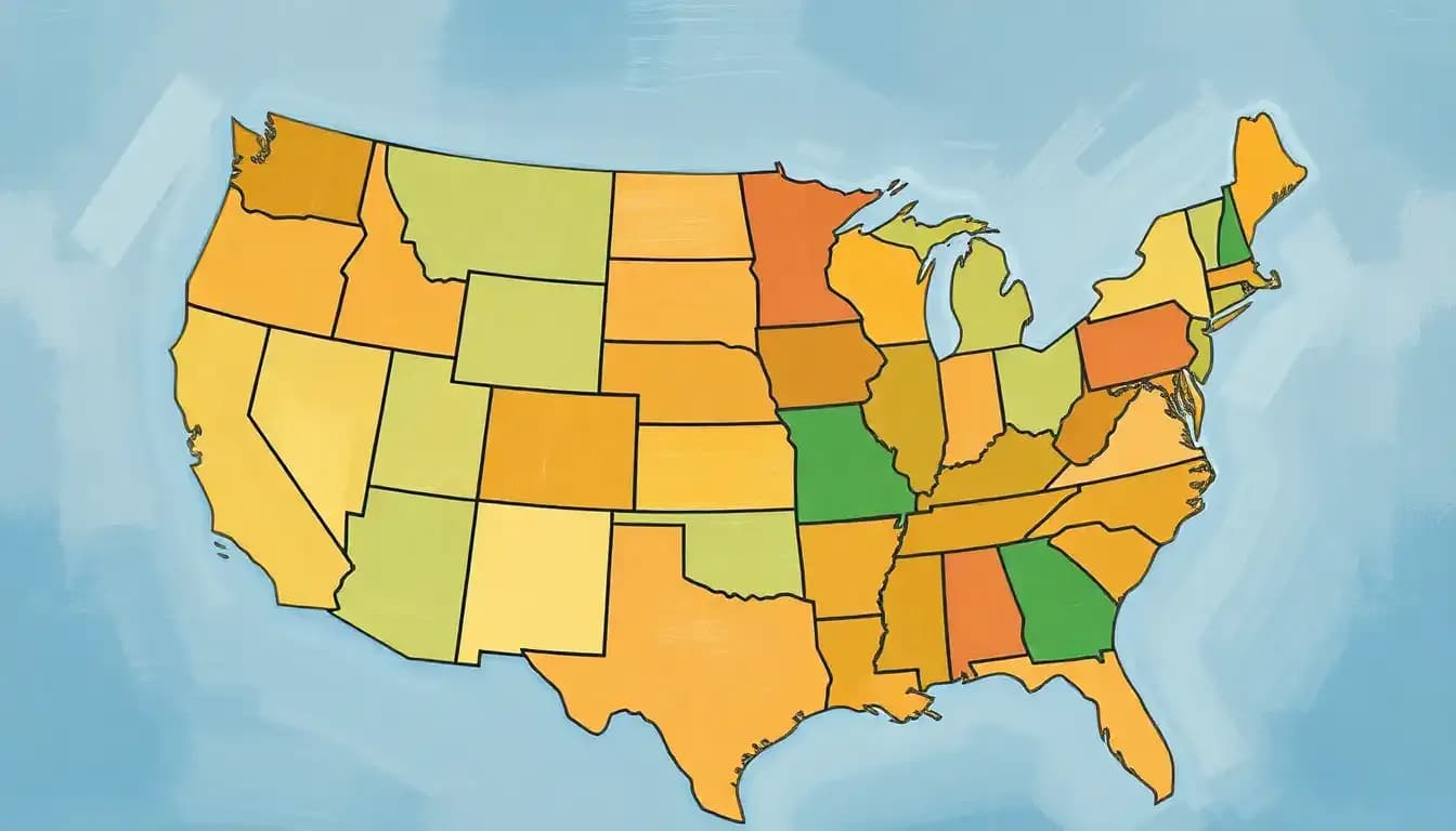
Picture this: you’re standing in front of a giant map of the United States, but instead of state borders, you see a patchwork of colors representing different cost of living levels. This, my friend, is the HCOL map concept in a nutshell. It’s a visual representation of how expensive it is to maintain a certain standard of living across various regions of the country.
The Big Spenders: Factors That Drive Up the Cost of Living
Now, let’s talk about the culprits behind those sky-high expenses in HCOL areas. It’s not just one thing that makes these places pricey – it’s a perfect storm of several factors working together.
First up, we have housing expenses. In HCOL Cities: Navigating High Cost of Living Urban Areas, you’ll find that real estate prices can be astronomical. We’re talking about places where a tiny studio apartment might cost more than a spacious family home in other parts of the country. Rent and mortgage payments in these areas can easily gobble up a significant chunk of your income.
But it doesn’t stop there. Transportation costs in HCOL areas can also put a dent in your wallet. Whether you’re shelling out for expensive public transit passes or dealing with high gas prices and parking fees, getting around in these areas isn’t cheap.
And let’s not forget about food and grocery prices. In HCOL regions, even a simple trip to the supermarket can feel like a luxury shopping spree. From organic produce to artisanal bread, everything seems to come with a premium price tag.
Healthcare expenses are another major factor. In HCOL areas, medical services, insurance premiums, and prescription drugs often come with hefty price tags. It’s enough to make you want to bubble-wrap yourself to avoid any potential injuries!
Last but not least, taxes and utilities in HCOL areas can be a real pain in the pocket. Higher income taxes, property taxes, and steeper utility bills all contribute to the overall cost of living.
The Usual Suspects: Top HCOL Areas in the United States
Now that we’ve covered the “why,” let’s talk about the “where.” Some areas in the U.S. are notorious for their high cost of living. These places might offer amazing opportunities and experiences, but they also demand a pretty penny in return.
First on our list is the Big Apple itself – New York City and its surrounding areas. From the bustling streets of Manhattan to the trendy neighborhoods of Brooklyn, living in NYC often means paying top dollar for, well, just about everything. But hey, if you can make it there, you can make it anywhere, right?
Next up, we have the San Francisco Bay Area. Home to tech giants and sourdough bread, this region is known for its astronomical housing prices and overall high cost of living. It’s not uncommon to hear stories of software engineers living in shared apartments despite earning six-figure salaries.
Moving down the coast, we hit Los Angeles and Southern California. While it might not be quite as expensive as San Francisco, LA still packs a punch when it comes to living costs. But with year-round sunshine and beaches, some might argue it’s worth every penny.
On the East Coast, the Washington D.C. metropolitan area stands out as another HCOL hotspot. Between government jobs, lobbying firms, and a vibrant cultural scene, the nation’s capital attracts many high-earning professionals – and high prices follow suit.
Rounding out our top five is Boston and the New England region. Known for its prestigious universities and thriving healthcare industry, this area combines historic charm with modern-day expense. Just be prepared to pay a premium for that clam chowder!
Mapping It Out: Tools and Resources for Understanding HCOL
Now, you might be wondering, “How can I navigate this complex landscape of living costs?” Fear not! There are plenty of tools and resources available to help you understand and compare HCOL areas.
Online HCOL map resources are a great place to start. Websites like Numbeo and Expatistan offer interactive maps and cost of living comparisons between cities worldwide. These can give you a quick visual overview of how expenses stack up in different areas.
For those who love hard data, government statistics are your best friend. The U.S. Bureau of Labor Statistics provides detailed information on consumer expenditures across different regions. It’s not the most exciting bedtime reading, but it’s packed with valuable insights.
Cost of living calculators are another handy tool in your HCOL toolkit. These nifty online gadgets allow you to compare living expenses between different cities. Just plug in your current location, your potential new home, and your income, and voila! You’ll get a breakdown of how your purchasing power might change.
Don’t forget to keep an eye on real estate market trends, too. Websites like Zillow and Redfin offer up-to-date information on housing prices, rent trends, and market forecasts. These can be particularly useful if you’re considering a move to a High Income Areas: Exploring the Most Affluent Neighborhoods in America.
Living Large (or Small) in HCOL Areas: Impact on Career and Lifestyle
Living in an HCOL area isn’t just about higher expenses – it can have a significant impact on your career and lifestyle choices too. Let’s break it down.
First off, salary expectations in HCOL areas tend to be higher. Employers often offer “cost of living adjustments” to compensate for the increased expenses. However, don’t assume that a higher salary automatically means more disposable income. Sometimes, the increased costs can outweigh the pay bump.
Work-life balance is another crucial consideration. HCOL areas often come with longer commute times and higher-stress work environments. You might find yourself working longer hours to justify that higher salary, leaving less time for personal pursuits.
But here’s where things get interesting: the rise of remote work is shaking up the HCOL landscape. With more companies embracing work-from-home policies, some folks are choosing to earn big-city salaries while living in more affordable areas. It’s like having your cake and eating it too!
If you do decide to take the plunge and live in an HCOL area, there are strategies to make it work. Sharing housing costs with roommates, mastering the art of budgeting, and taking advantage of free local amenities can help stretch your dollars further. It might mean sacrificing some luxuries, but for many, the opportunities and experiences of HCOL areas make it worthwhile.
Crystal Ball Gazing: Future Trends in HCOL Areas
So, what does the future hold for HCOL areas? While I haven’t perfected my fortune-telling skills just yet, we can make some educated guesses based on current trends.
Economic factors will continue to play a significant role in shaping HCOL trends. Things like job market growth, inflation rates, and global economic conditions can all influence which areas become more or less expensive over time.
The shift towards remote work could potentially reshape the HCOL map as we know it. We might see traditionally expensive urban centers become more affordable as people move to smaller cities or rural areas. On the flip side, some previously affordable areas might see cost increases as they attract remote workers with higher salaries.
Urban development will also impact cost of living trends. As cities invest in infrastructure, public transportation, and amenities, it could drive up living costs in certain areas. However, smart urban planning could also help create more affordable housing options.
Keep an eye out for emerging HCOL areas, too. Cities with growing tech scenes, booming cultural sectors, or improving quality of life metrics could see cost of living increases in the coming years. Today’s affordable hidden gem could be tomorrow’s High Income Zip Codes Near Me: Discovering Affluent Neighborhoods in Your Area.
Wrapping It Up: Why HCOL Maps Matter
As we come to the end of our HCOL journey, let’s recap why understanding these cost of living variations is so important. HCOL maps and data provide valuable insights that can inform major life decisions. Whether you’re considering a job offer in a new city, planning for retirement, or just trying to budget more effectively, having a grasp on cost of living differences is crucial.
For individuals, this knowledge can help you make informed choices about where to live, work, and invest. It can guide your salary negotiations, help you set realistic financial goals, and even influence your career path.
For businesses, understanding HCOL areas is equally important. It can inform decisions about where to locate offices, how to set salaries, and how to adjust pricing strategies across different markets.
The key takeaway? Stay informed about cost of living trends. The financial landscape is constantly evolving, and what’s true today might not be true tomorrow. Keep an eye on those HCOL maps, stay up-to-date with economic news, and don’t be afraid to crunch the numbers when making big life decisions.
Remember, living in an HCOL area doesn’t have to mean financial struggle. With the right information and strategies, you can navigate these pricey waters and potentially even thrive. Who knows? You might find yourself living it up in a High Income Housing: Luxury Living in Premium Real Estate Markets sooner than you think!
So, the next time you look at your paycheck and wonder where it all goes, just remember: it’s not you, it’s your zip code. But armed with knowledge about HCOL areas, you’re now better equipped to make that paycheck work for you, no matter where you choose to call home.
References:
1. U.S. Bureau of Labor Statistics. (2021). Consumer Expenditure Surveys. https://www.bls.gov/cex/
2. Numbeo. (2023). Cost of Living. https://www.numbeo.com/cost-of-living/
3. Zillow Research. (2023). Housing Data. https://www.zillow.com/research/
4. Pew Research Center. (2022). The State of the American Workplace.
5. Urban Land Institute. (2023). Emerging Trends in Real Estate.
6. Federal Reserve Bank of St. Louis. (2023). Economic Research. https://fred.stlouisfed.org/
7. National Association of Realtors. (2023). Housing Statistics. https://www.nar.realtor/research-and-statistics
8. U.S. Census Bureau. (2023). American Community Survey. https://www.census.gov/programs-surveys/acs
9. Brookings Institution. (2022). Metro Monitor: Tracking Growth, Prosperity, and Inclusion in the 100 Largest U.S. Metropolitan Areas.
10. McKinsey & Company. (2023). The Future of Work in America: People and Places, Today and Tomorrow.